In this sample analysis notebook, we will analysis the data from the Crab pulsar as observed with LAXPC We will extract the lightcurves, powerspectrum and pulse profile of the pulsar.
A typical LAXPC observation has data from 3 detectors LAXPC 1-3 and for each detector (also called units), the photons are detected on multiple layers. For faint sources, it is advisable to extract data from layer 1 as it has the least contribution from the background events.
The notebook is designed for LAXPC observation processed using Format (A) software as available on AstroSat Science support cell. A tutorial for processing the LAXPC data can be found here
Imports
[ ]:
import stingray
from stingray import EventList, Powerspectrum, AveragedPowerspectrum
from astropy.io import fits
import matplotlib.pyplot as plt
import numpy as np
import stingray.pulse as stp
import pytest
import os
Loading the event file.
To proceed further, download the data set from Zenodo and unzip the files. There should be two files: 1. Event file and 2. GTI
[ ]:
fpath = os.getcwd()         # Update this path to the directory where the downloaded and extracted files are kept.
evt_fname = os.path.join(fpath, "level2.event.fits")
gti_fname = os.path.join(fpath, "usergti.fits")
ev = EventList.read(evt_fname, 'hea', additional_columns=["Layer"])
/home/yash/1.Cagliari/stingray_dev/stingray_git/stingray/io.py:959: UserWarning: HDU EVENTS not found. Trying first extension
  warnings.warn(f"HDU {hduname} not found. Trying first extension")
/home/yash/1.Cagliari/stingray_dev/stingray_git/stingray/io.py:1060: UserWarning: No valid GTI extensions found.
Error: list index out of range
GTIs will be set to the entire time series.
  warnings.warn(
Oops. There are some warnings due to differences in the inherent data structure of the LAXPC event file but it seems to be have read correctly. One of the errors was the absence of the GTI extension, so we load the GTI manually, as follows.
[3]:
gti = stingray.gti.load_gtis(gti_fname)
ev.apply_gtis(new_gti=gti)
[3]:
<stingray.events.EventList at 0x7d023a9c2590>
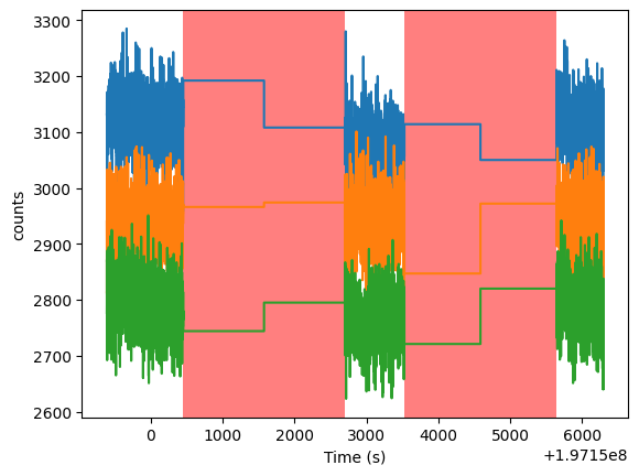
Filtering based on Units
In this exercise, we will extract events from individual units, generate lightcurves and plot them.
[4]:
# Filtering the events based on the detector ID
unit1 = ev.filter_detector_id(1)
unit2 = ev.filter_detector_id(2)
unit3 = ev.filter_detector_id(3)

lc_unit1 = unit1.to_lc(dt=1)
lc_unit1.apply_gtis()
lc_unit2 = unit2.to_lc(dt=1)
lc_unit2.apply_gtis()
lc_unit3 = unit3.to_lc(dt=1)
lc_unit3.apply_gtis()


lc_unit1.plot()
lc_unit2.plot(plot_btis=False)
lc_unit3.plot(plot_btis=False)
# plt.show()
/home/yash/1.Cagliari/stingray_dev/stingray_git/stingray/events.py:696: UserWarning: The input event list has a time resolution of 9.99999975e-06. Using a multiple of that as dt (0.999999975).
  warnings.warn(
[4]:
<Axes: xlabel='Time (s)', ylabel='counts'>
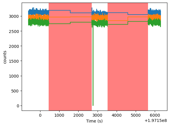
[5]:
min_counts = 2500
new_gti = stingray.gti.create_gti_from_condition(lc_unit1.time, lc_unit1.counts>min_counts)
merged_gti = stingray.gti.cross_two_gtis(new_gti, gti)
# print (new_gti, gti, merged_gti)

unit1.apply_gtis(merged_gti)
lc_unit1 = unit1.to_lc(dt=1)
lc_unit1.apply_gtis()
lc_unit1.plot()
unit2.apply_gtis(merged_gti)
lc_unit2 = unit2.to_lc(dt=1)
lc_unit2.apply_gtis()
lc_unit2.plot(plot_btis=False)
unit3.apply_gtis(merged_gti)
lc_unit3 = unit3.to_lc(dt=1)
lc_unit3.apply_gtis()
print (lc_unit3.gti)
lc_unit3.plot(plot_btis=False)
[[1.97149389e+08 1.97150455e+08]
 [1.97152699e+08 1.97152763e+08]
 [1.97152768e+08 1.97153530e+08]
 [1.97155643e+08 1.97156299e+08]]
[5]:
<Axes: xlabel='Time (s)', ylabel='counts'>
Now the light curve for each Unit is well behaved. We also see slightly different count rates in each unit.
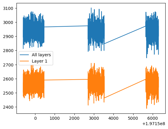
Filtering based on layer
In this we will extract based on a single layer and all layers for a particular unit and compare the lightcurves
[6]:
unit2_layer1 = unit2.apply_mask((unit2.layer==1))
lc_unit2_layer1 = unit2_layer1.to_lc(dt=1)
lc_unit2_layer1.apply_gtis()

plt.plot(lc_unit2.time, lc_unit2.counts, label="All layers")
plt.plot(lc_unit2_layer1.time, lc_unit2_layer1.counts, label='Layer 1')
plt.legend()
[6]:
<matplotlib.legend.Legend at 0x7d023a8ae590>
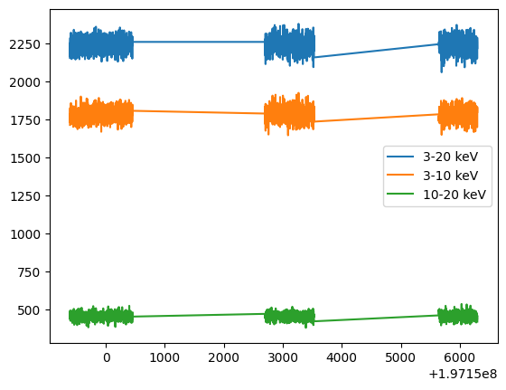
Energy dependent lightcurves
Here we will extract energy dependent lightcurves
[7]:
unit2_layer1_soft = unit2_layer1.filter_energy_range([3,10])
unit2_layer1_hard = unit2_layer1.filter_energy_range([10,20])
unit2_layer1_full = unit2_layer1.filter_energy_range([3,20])


soft_lc = unit2_layer1_soft.to_lc(1)
hard_lc = unit2_layer1_hard.to_lc(1)
full_lc = unit2_layer1_full.to_lc(1)
soft_lc.apply_gtis()
hard_lc.apply_gtis()
full_lc.apply_gtis()

plt.plot(full_lc.time, full_lc.counts, label="3-20 keV")
plt.plot(soft_lc.time, soft_lc.counts, label="3-10 keV")
plt.plot(hard_lc.time, hard_lc.counts, label="10-20 keV")
plt.legend()
[7]:
<matplotlib.legend.Legend at 0x7d023a7985d0>
Search of pulsations and folding
Since the source we are analysing is a pulsar, we can search for pulsations. Here are some steps for the same
Generate a power-density spectrum and look for peaks.
Epoch fold search on the data
Epoch folding of the best-fit period.
Power spectrum
[8]:
avg_pds = AveragedPowerspectrum.from_events(unit2, dt = 0.001, segment_size=1.024, gti=merged_gti, norm="leahy")
pds =  Powerspectrum.from_events(unit2, dt = 0.001,  gti=merged_gti, norm="leahy")
/home/yash/1.Cagliari/stingray_dev/stingray_git/stingray/events.py:696: UserWarning: The input event list has a time resolution of 9.99999975e-06. Using a multiple of that as dt (0.0009999999750000001).
  warnings.warn(
2486it [00:00, 5320.14it/s]
/home/yash/1.Cagliari/stingray_dev/stingray_git/stingray/events.py:696: UserWarning: The input event list has a time resolution of 9.99999975e-06. Using a multiple of that as dt (0.0009999999750000001).
  warnings.warn(
/home/yash/1.Cagliari/stingray_dev/stingray_git/stingray/utils.py:2158: UserWarning: Cannot calculate the histogram with the numba implementation. Trying standard numpy.
  warnings.warn(
[9]:
plt.plot(pds.freq, pds.power, alpha=0.5, c='C0', label='PDS')
plt.plot(avg_pds.freq, avg_pds.power, alpha=0.5, c='k', label='PDS after averaging')
plt.legend()
plt.yscale('log')
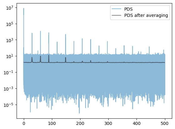
We can see there are a plethora of peaks. Most of them are harmonics peaks due to the non-sinusoidal nature of the pulse profile. And the effect of averaging the PDS is also evident. The noise reduces, but the peaks broaden as we are increasing the frequency resolution, leading to a broader peak.
The spin frequency of Crab is ~29 Hz and therefore to get an accurate period, we can use epoch folding search
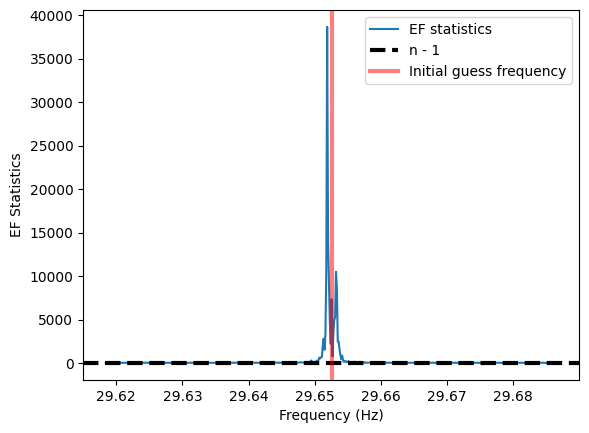
Epoch folding search
[10]:
# To determine the guess period, lets take the central frequency of the peak in the PDS

short_freq_indices = np.where((pds.freq>25) & (pds.freq<35))

initial_guess_freq = pds.freq[short_freq_indices][np.argmax(pds.power[short_freq_indices])]
print ("Initial guess frequency:", initial_guess_freq)


# We search a grid of frequencies around the guess frequency.
df_min = 2e-3
oversampling=15
df = df_min / oversampling
n_freq = 256
frequencies = np.arange(initial_guess_freq - n_freq * df, initial_guess_freq + n_freq * df, df)
nbin = 32

freq, efstat = stp.search.epoch_folding_search(unit2.time, frequencies, nbin=nbin)

best_estimate_freq = freq[np.argmax(efstat)]
print (f"Best fitting period: {best_estimate_freq}")
plt.plot(freq, efstat, label='EF statistics')
plt.axhline(nbin - 1, ls='--', lw=3, color='k', label='n - 1')
plt.axvline(initial_guess_freq, lw=3, alpha=0.5, color='r', label='Initial guess frequency')
plt.xlabel('Frequency (Hz)')
plt.ylabel('EF Statistics')
plt.legend()
Initial guess frequency: 29.652533302818394
Best fitting period: 29.651866636151947
[10]:
<matplotlib.legend.Legend at 0x7d02399b5610>
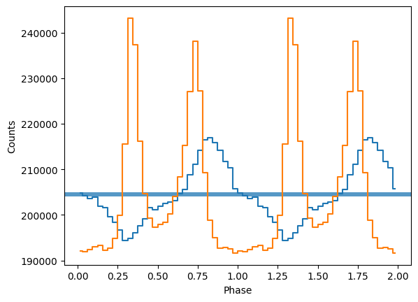
Folding on the guess and best period
[11]:
nbin=32
ph, profile, profile_err = stp.pulsar.fold_events(unit2_layer1.time, initial_guess_freq, nbin=nbin)
_ = stp.search.plot_profile(ph, profile)

ph_best, profile_best, profile_err = stp.pulsar.fold_events(unit2_layer1.time, best_estimate_freq, nbin=nbin)
_ = stp.search.plot_profile(ph_best, profile_best)